Radschool Association Magazine - Vol 23

Page 4

Print this page

Computers and stuff

Sam Houliston

The hidden calculator.

Did you know that MS-Word has an inbuilt calculator? If you’re a long time user, dating back to Word 97, you probably do, but if you’re new to Word you probably don’t. To use it, you first have to resurrect it. You do that like this:-

Word 2007

• Right-click the Quick Access toolbar and select Customize Quick Access Toolbar from the pop-up menu.

• Make sure For All Documents is selected in the Customize Quick Access Toolbar drop-down box.

• In the Choose Commands From drop-down box, select Commands Not In The Ribbon. (Side note: Perusing this list is highly educational for old-time Word users pining for lost commands.)

• Locate Calculate in the list and double-click it to add it to the list of Quick Access commands, then click OK.

Word XP/2003

• Click Tools then click Customize.

• Click the Commands tab in the Customize dialog.

• In the Categories list click Tools and in the Commands list scroll to “Tools Calculate”.

• Click and drag the Tools Calculate command onto any of your toolbars.

Using the Calculator

With the Calculator now on the toolbar, you're ready to give it a whirl.

• Enter a simple formula in a Word document

• Select the entire text

• Click your new Calculator button.

Word will work out the result, display it on the status bar and copy the number into the clipboard for you to paste.

Percentages: %   (89765*23.5%)  

Exponentiation:  ^    7^4

Calculating a cube root: 1728^(1/3)

If you don't include brackets, the calculator performs operations in this order:

1. percentage

2. power and root

3. multiplication and division

4. addition and subtraction

Software checker

It is very important that you keep your software up to date by installing the software manufacturer’s security updates and patches. Hackers can and do insert malicious code into software using a technique called cross-site scripting, or XSS. Software manufacturers know this and, as soon as hackers have written code to infect their software, the manufacturers  bring out an update to close off their software’s vulnerable ‘bit’. You can check to see if the software on your computer is the latest and safest version by using a free Software Checker. Get your copy HERE.  The Software Checker will check all your programs and advise which, if any, are subject to attack. If it finds any, it will also show you where to get the update.

Broadband Speed

There are several web sites that test internet connection speed. One good site is http://www.speedtest.net

Spam – at last there’s an answer.

 If, like everyone else, you’re sick to the back teeth with all that Spam that does nothing but clog up your in-box,  well, now there is an answer. There’s a great little program that automatically gets rid of all that spam for you and what’s more, it’s very easy to use and it’s almost  FREE!!!. It’s called Comodo and you can get your free copy HERE.

What's the price? Well, it doesn't cost any thing monetary wise, but people that aren't white-listed with Comodo on your PC, who try to email you, will get a one-off request to confirm that they are legit. Spammers will never reply to this because they don't give real reply-to addresses - they will never get the request. But your friend who emailed may be daunted by the request and fail to respond. So if you want to use Comodo take the trouble to white-list in advance as much of your address book as possible. 

Another trick you can try to reduce spam is to open a gmail (Google mail) account and if your provider supports email forwarding and multiple addresses, forward your mail to your gmail address and set up gmail to forward to an undisclosed second address with your provider, which is the one you read your email from (but set up Outlook or Thunderbird to use your normal email address on outgoing mail). Nearly all of the spam will be captured in the gmail spam folder and you won't see it.

Or you could just use gmail.

Wireless on the move.

If you’re using a wireless laptop to connect to the internet while staying at a hotel, or perhaps you’re using one of your local Council’s free Wi-Fi access points, then you should be very very careful. Odds are, if you check your computer’s “Network Places” you will find a heap of computers all hooked up in your workgroup. This is because nearly everyone accepts the default Microsoft network name and is running under the name ‘MSHOME.'

There’s an old saying, “if the enemy is in range, then so are you”, and this works with networked computers too. As well as you being able to see everyone else’s shared folders, anyone else on the network would be able to see yours, so it’s a good idea to rename your workgroup to something specific as this will keep out the curious and the opportunists. It won’t keep out the determined, locks only keep out honest people anyway, so you may also wish to remove documents from your shared folders before going out!

Excel References.

This article appeared in "Office Watch", a web based newsletter. I thought it so useful it has been reproduced here.

When you refer to a cell in an Excel formula, you can use any of three different types of reference: Relative, Absolute and Mixed.

Relative cell references are the most commonly used. A relative cell reference in a formula is based on the position of the formula's cell relative to the cell to which it refers. That means if you move the formula cell, or copy it elsewhere, the reference changes. You denote a relative reference simply by using the cell's column letter followed by its row number: A1. A simple formula that uses relative cell references to add the numbers in cells B1 through B9 is:

=SUM(B1:B9)

If you place this formula in cell B10 and then copy it across from B10 to C10, Excel makes the sensible assumption that you want to total the values in the same relative positions in column C - that is, cells C1 to C9 - and so it automatically adjusts the formula to read:

=SUM(C1:C9)

An absolute reference refers to a cell in a fixed location. Such references come in handy when you want to refer consistently to the same cell, or range of cells, throughout a worksheet. For example, if you use a worksheet to estimate a mileage allowance for business travel, you could put the allowance rate per mile in cell D2 and then use an absolute reference to that cell anywhere you use a formula based on the mileage rate. To indicate an absolute reference use dollar signs, thus: $D$2.

Name that Cell.

You can make life easier for yourself by naming a cell or range of cells. This is particularly handy when you want to refer to a certain cell repeatedly in formulas. When you name a cell, Excel automatically makes it an Absolute reference.

For example, to name our mileage rate cell in Excel 2007:

1. Right-click the cell and select "Name A Range" from the pop-up menu.

2. Type a name in the Name box, such as MileageRate and click OK. Although you can't include spaces in the name, you can use underscores (Mileage_Rate), periods/full stops (Mileage.Rate) or slashes (Mileage\Rate). Excel ignores the case, but it can make your worksheets more readable if you mix lower  and uppercase.

To name the cell in Excel 2003:

1. Click the cell.

2. Click Insert -> Name -> Define.

3. Type in the name, MileageRate, and click OK.

Once you've named the cell, you can use its name in any formula, thus: =E7*MileageRate

As you define the name, notice the value in the Refers To box. You'll see the full absolute reference consists of the worksheet name followed by an exclamation mark and the absolute cell reference, for example: ='Travel Expenses'!$D$2. That means you can use the named reference - in our case, MileageRate - in any worksheet in your workbook, not just the current worksheet.

That's great, but what if you've set your workbook up with a separate worksheet for each employee and each of those employees has a different mileage rate? In that case, you won't want a reference to MileageRate on Mildred's worksheet grabbing the value from Darren's worksheet.

In Excel 2003, you deal with this situation by specifying the worksheet when defining a name: in the Name box, first type the current worksheet's name, followed by an exclamation mark, followed by your chosen cell name. For example: Darren!MileageRate. Excel 2007, makes this easier by including a Scope box in the New Name dialog: when you define the name, select the current worksheet from the drop-down Scope box to restrict the reference to the current sheet, and Excel will name it appropriately.

If you ever need to delete a cell/range name,

In Excel 2007:

1. On the Formulas tab click Name Manager.

2. In the Name Manager dialog, click the name you want to delete and click the Delete button.

in Excel 2003:

1. Click Insert -> Name -> Define.

2. In the Define Name dialog, click the name you want to delete then click the Delete button.

When you refer to a cell in an Excel formula, you can use any of three different types of reference: relative, absolute and/or mixed. Mixed references are a combination of relative and absolute: for example D$2 where the column “D” is relative and the row “2” fixed (absolute), or $D2 where the column “D” is fixed and the row “2” relative.

When would you need such a reference? One case is when you create any table where the values are derived by multiplying the x axis by the y axis. A multiplication table is the simplest example of this.

The easiest way to get a feel for mixed references is to give them a try:

1. Place the values 1 through 12 across in cells B2 to M2. This is the x axis of your multiplication table.

2. Place the values 1 through 12 down in cells A3 to A14. This is the y axis of your multiplication table.

3. In the top, left-most cell of the results grid, cell B3, enter the formula: =B$2*$A3.

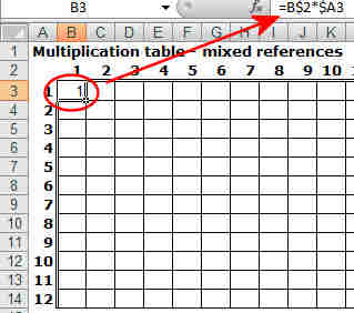
Excel cell references - Mixed References 1.

1. Copy that formula down and then across to include the entire table.

This formula translates as: “Multiply the value in row 2, column x by the value in column A, row y. For the first cell referenced in the formula, the row remains constant (row 2, the x axis where you placed the values 1 through 12) while the column changes. For the second cell reference, the column remains constant (column A, the y axis where you placed the values 1 through 12), while the row changes. No matter where you click in the table, you'll see row 2 and column A referenced in the formula bar, while the other values vary.

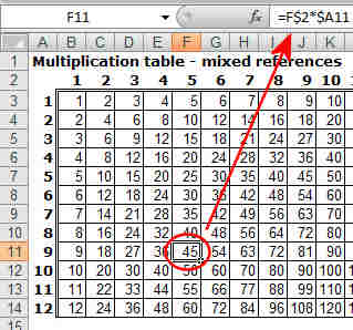
Excel cell references - Mixed References 2.

CHANGING REFERENCE TYPES.

If you find you've used the wrong type of reference in a formula, Excel offers a shortcut for changing the reference:

1. Click the offending cell.

2. In the formula bar, click the incorrect cell reference and press F4. Each time you press F4, Excel will cycle the reference through relative -> absolute -> mixed (relative/absolute) -> mixed (absolute/relative).

3. Repeat this process for each incorrect reference in the formula.

Windows XL Service Pack 3

It seems there are some serious problems involving Service Pack 3 for Windows XP.  The problems with XP SP3 include AMD-based Hewlett-Packard desktop computers constantly rebooting and Symantec antivirus products developing strange behaviours. You can read more about it HERE

My advice - wait on installing XP SP3 if you don't have some urgent need for it.

The quickest way for a parent to get a child's attention is to sit down and look comfortable.